广义线性模型中的逻辑斯蒂回归

其实题目不太准确,这篇短文介绍的是二项分布线性模型, 也就是当响应变量为01时的线性模型,例如物种是否出现,病人是否需要住院,学生是否成功考入大学,英语四六级成绩是否及格等。逻辑斯蒂回归模型,是二项分布线性模型中的一种,也是最广泛的一种。

事情还要从1935年说起。那一年,英国伦敦大学学院的C.I. Bliss 在《Annals of Applied Biology》上发表论文The Calculation of the Dosage**-**Mortality Curve。这篇论文的表4,就是现在广泛用于逻辑斯蒂回归教学的beetle数据。该数据是C.I. Bliss从Strand在1930年发表的论文中摘出来的。

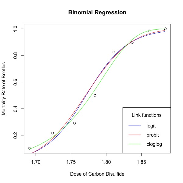
Bliss的这篇论文主要以杂拟谷盗**(Tribolium confusum)**为例,系统介绍拟合存活比例曲线的方法。杂拟谷盗是一种粮食害虫。当时生物学家将481只杂拟谷盗分成8组,每一组分别在暴露在不同浓度的二硫化碳5小时,之后记录每个组有多少只甲虫死了。由于甲虫对二硫化碳的反应只有两种可能,要么存活,要么死亡,所以这个数据集是典型的二项分布数据。

在这篇论文中,Bliss提出了一种连接函数,也就是事件发生与否,用转换以后的正态分布累计曲线去估算,称为Probit。实际上,二项分布线性模型的连接函数有三种,分别为logit, probit以及cloglog。 logit、probit以及cloglog都是统计变换,目的是将二项分布数据转换为一种形式,以便能用线性模型估计直接估计模型的参数。其中最常见的为logit,使用logit连接函数的二项分布回归称为逻辑斯蒂回归。logit是事件发生与是否发生的比例 (odds)的对数值,形为log**(y/(1-y)),称为log odds。cloglog是complementary log log的缩写,是将响应变量进行两次log变换, 公式为log(-log(1-y))**。 cloglog常用来拟合数据出现大量极端数值的数据, 例如,大样地的幼苗的负密度制约研究中,部分胸径等级的树苗只有很少一部分死亡,用cloglog能较准确捕捉到与树苗死亡相关性较强的环境因子, 如同种密度制约、光环境等。

下面用R代码演示如何进行二项分布回归,分别用logit, probit以及cloglog三种连接函数。

1
2
3
4
5
6
7
8
9
10
11
12
13
14
15
16
17
18
19
20
21
22
23
24
25
26
27
28
29
30
31
32
33
34
35
36
37
38
39
40
41
42
43
44
45
46
47
48
49
50
51
52
53
54
55
56
57
58
59
60
61
62
63
64
65
66
67
68
69
70
71
72
73
74
75
library(broom)
####表格形式的数据
####tabular form
####数据来源www.stat.ualberta.ca/~kcarrier/STAT562/comp_log_log
####beetle
####   LOGDOSE     NUMBER_OF_BEETLES  NUMBER_KILLED  COMP_LOG_LOGPROBITLOGIT
####1   1.691                59             6          5.7   3.4 35.0
####2   1.724                60            13         11.3  10.7  9.8
####3   1.755                62           18         20.9   23.422.4
####4   1.784                56            28         30.3  33.8 33.9
####5   1.811                63            52         47.7  49.6 50.0
####6   1.837                59            53         54.2  53.4 53.3
####7   1.861                62            61         61.1  59.7 59.2
####8   1.884                60            60         59.9  59.2 58.8
####>
####二硫化碳的浓度
LOGDOSE          <-c(1.6911.7241.7551.7841.8111.8371.8611.884 )
####各小组杂拟谷盗的头数
NUMBER_OF_BEETLES<-c(59,    60,    62,    56,    63,    59,    62,    60    )    
####杂拟谷盗经过二硫化碳熏蒸5小时后,死亡的个体数
NUMBER_KILLED    <-c(6,     13,    18,    28,    52,    53,    61,    60    )
####合并成一个数据框
beetle<-data.frame(NUMBER_OF_BEETLES,NUMBER_KILLED, LOGDOSE)
####第一种方法,数据表格式
####调用glm函数,注意连接函数的选择
mod_logit  <-glm(cbind(NUMBER_KILLED, NUMBER_OF_BEETLES -NUMBER_KILLED)~LOGDOSE,data=beetle,  family=binomial(link="logit") )
mod_probit <-glm(cbind(NUMBER_KILLED, NUMBER_OF_BEETLES -NUMBER_KILLED)~LOGDOSE,data=beetle,  family=binomial(link="probit"))
mod_cloglog<-glm(cbind(NUMBER_KILLED, NUMBER_OF_BEETLES -NUMBER_KILLED)~LOGDOSE,data=beetle,  family=binomial(link="cloglog"))
####Showing significance of the variables
tidy(mod_logit )

\## term estimate std.error statistic p.value
\##1 (Intercept) -60.74013 5.181870 -11.72166 9.871561e-32
\##2 LOGDOSE 34.28593 2.913213 11.76911 5.631446e-32

tidy(mod_probit)

\## term estimate std.error statistic p.value
\##1 (Intercept) -34.95614 2.648984 -13.19605 9.245343e-40
\##2 LOGDOSE 19.74103 1.488046 13.26640 3.625628e-40

tidy(mod_cloglog)

\## term estimate std.error statistic p.value
\##1 (Intercept) -39.52224 3.235649 -12.21463 2.596958e-34
\##2 LOGDOSE 22.01474 1.796996 12.25085 1.662370e-34

\####Showing AIC et al.
glance(mod_logit )

\## null.deviance df.null logLik AIC BIC deviancedf.residual
\##1 284.2024 7 -18.65681 41.31361 41.4725 11.11558 6

glance(mod_probit)

\## null.deviance df.null logLik AIC BIC deviancedf.residual
\##1 284.2024 7 -18.0925 40.18499 40.34388 9.986957 6

glance(mod_cloglog)

\## null.deviance df.null logLik AIC BIC deviancedf.residual
\##1 284.2024 7 -14.85619 33.71237 33.87126 3.514334 6

\####绘图Visualisingthe results
mortality_rate<-beetle$NUMBER_KILLED/beetle$NUMBER_OF_BEETLES
dose<-beetle$LOGDOSE
plot(mortality_rate~dose,xlab="Dose of Carbon Disulfide",ylab="MortalityRate of Beetles",main="BinomialRegression")
LOGDOSE_new=seq(min(dose),max(dose),length.out=200)
mod_logit_line <-predict(mod_logit,newdata=data.frame(LOGDOSE=LOGDOSE_new), type="response")
lines(mod_logit_line~LOGDOSE_new,col="blue")
mod_probit_line <-predict(mod_probit,newdata=data.frame(LOGDOSE=LOGDOSE_new), type="response")
lines(mod_probit_line~LOGDOSE_new,col="red")
mod_cloglog_line <-predict(mod_cloglog,newdata=data.frame(LOGDOSE=LOGDOSE_new), type="response")
lines(mod_cloglog_line~LOGDOSE_new,col="green")
legend("bottomright",title="Linkfunctions",legend=c("logit","probit","cloglog"),lty=c(1,1,1),col=c("blue","red","green"))

img

1
2
3
4
5
6
7
8
9
10
11
12
13
14
15
16
17
18
19
20
21
22
23
24
25
26
27
28
29
30
31
32
33
34
35
36
37
38
39
40
41
42
43
44
45
46
47
48
49
50
51
52
53
54
55
56
57
58
59
60
61
62
63
64
65
66
67
68
69
70
71
72
73
74
75
76
77
78
79
80
81
\#####第二种方法,每个个体生存状态的长数据格式。glm是可以接受这种格式的。
\#####按照个体来计
dose_surived<-
c(rep(1.691,59-6),
rep(1.724,60-13),
rep(1.755,62-18),
rep(1.784,56-28),
rep(1.811,63-52),
rep(1.837,59-53),
rep(1.861,62-61),
rep(1.884,60-60))
dose_dead<-c(
rep(1.691, 6),
rep(1.724,13),
rep(1.755,18),
rep(1.784,28),
rep(1.811,52),
rep(1.837,53),
rep(1.861,61),
rep(1.884,60))
status_survived<-c(
rep("alive",59-6),
rep("alive",60-13),
rep("alive",62-18),
rep("alive",56-28),
rep("alive",63-52),
rep("alive",59-53),
rep("alive",62-61),
rep("alive",60-60))
status_dead<-c(
rep("dead", 6),
rep("dead",13),
rep("dead",18),
rep("dead",28),
rep("dead",52),
rep("dead",53),
rep("dead",61),
rep("dead",60)
)

dose_long<-c(dose_dead,dose_surived)
status <-as.factor(c(status_dead,status_survived))

incidence_mod_logit <-glm(status~dose_long,family=binomial(link="logit"))
incidence_mod_probit <-glm(status~dose_long,family=binomial(link="probit"))
incidence_mod_cloglog<-glm(status~dose_long,family=binomial(link="cloglog"))

\####Showing significance of the variables
tidy(incidence_mod_logit )

\## term estimate std.error statistic p.value
\##1 (Intercept) -60.74013 5.181834 -11.72174 9.861985e-32
\##2 dose_long 34.28593 2.913192 11.76920 5.625873e-32

tidy(incidence_mod_probit)

\## term estimate std.error statistic p.value
\##1 (Intercept) -34.95613 2.649010 -13.19592 9.261453e-40
\##2 dose_long 19.74102 1.488061 13.26627 3.631968e-40

tidy(incidence_mod_cloglog)

\## term estimate std.error statistic p.value
\##1 (Intercept) -39.52224 3.235632 -12.21469 2.594819e-34
\##2 dose_long 22.01474 1.796986 12.25092 1.660982e-34

\####Showing AIC et al.
glance(incidence_mod_logit )

\## null.deviance df.null logLik AIC BIC deviancedf.residual
\##1 645.441 480 -186.1771 376.3542 384.7059 372.3542 479

glance(incidence_mod_probit)

\## null.deviance df.null logLik AIC BIC deviancedf.residual
\##1 645.441 480 -185.6128 375.2255 383.5773 371.2255 479

glance(incidence_mod_cloglog)

\## null.deviance df.null logLik AIC BIC deviancedf.residual
\##1 645.441 480 -182.3765 368.7529 377.1046 364.7529 479